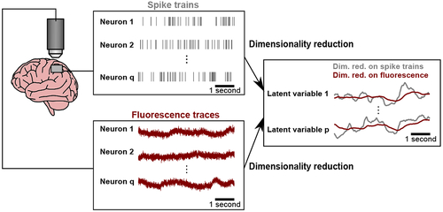
A key property of calcium imaging is the slow decay of the measured fluorescence (left panel, maroon) after each spiking event (left panel, grey). If ignored, the calcium decay could introduce temporal correlations in the estimated latent variables (right panel, maroon), where those temporal correlations would not be present had we estimated the latent variables from the underlying spike trains (right panel, grey).

(a) Each of the three classes of methods was applied to the simultaneously-recorded fluorescence of a population of neurons (y1,y2,…yq) to extract latent variables. Top, Approach 1: a standard dimensionality reduction method (e.g., LDS) applied directly to calcium imaging recordings, extracting corresponding low-dimensional latent variables at each time point (illustrated here with two dimensions, z₁ and z₂). Middle, Approach 2: deconvolution is applied separately to each neuron’s fluorescence trace to estimate its underlying spiking activity (s1,s2,…,sq). A standard dimensionality reduction method (e.g., LDS) is then applied to the estimated spiking activity to extract latent variables (z1 and z2). Bottom, Approach 3: A unified method (e.g., CILDS) that takes calcium imaging recordings as input and performs deconvolution and dimensionality reduction simultaneously to extract the latent variables (z1 and z2). (b) Cartoon depicting the intuition behind the difference between Approaches 2 and 3. Center column: a latent variable z (representing, for example, common input) is used to generate spike trains which, in turn, are used to generate fluorescence traces. Left column: Deconvolution is performed neuron by neuron (Approach 2, deconv-LDS), then an LDS is applied to the estimated spiking activity to extract latent variables. Right column: A unified method (Approach 3, CILDS) is applied to all neurons together to dissociate the calcium transients from the underlying shared spiking activity among neurons (i.e., the estimated latent variable). This is done by jointly performing deconvolution and dimensionality reduction, as illustrated by the the double arrows. Note that the estimated spiking activity is depicted here as spike trains for visual clarity, even though they are in fact continuous-valued time courses.

(a) Example simulated fluorescence traces (left panels) and estimated latent variables (right panels) for two combinations of experimental variables. Setting 1 corresponds to a latent timescale of 200ms, 94 neurons, calcium decay corresponding to GCaMP6f, and medium fluorescence noise (see Methods). Setting 2 is the same as Setting 1, but with high fluorescence noise. Each of the three dimensionality reduction approaches introduced in Fig. 2 (LDS, cyan; deconv-LDS, purple; CILDS, orange) is applied to the simulated fluorescence traces. The latent variables extracted by each method are then compared to the ground truth latent variables (black). (b-c) Accuracy of latent variables estimated by CILDS versus that of (b) LDS and (c) deconv-LDS. Accuracy is measured by the R² between each of the estimated and ground truth latent variables. Each point represents one latent variable on one trial, with a total of 2000 points for each setting, comprising 200 trials and 10 latent variables per trial. (d-g) Mean accuracy of latent variable recovery, as the (d) latent timescale, (e) number of neurons, (f) GCaMP6 indicator decay time constant, and (g) fluorescence noise level was varied. In each panel (d-g), one of the experimental variables was varied, while the other three variables were held constant at the Setting 1 values. The common point across the four panels is Setting 1 (shaded gray). Setting 2 (shaded purple) only appears in panel (g) because panels (d)-(f) correspond to medium rather than high fluorescence noise. The R² for other combinations of experimental variables are shown in Supplementary Fig. 1. Colored error bars indicate standard deviation, and black error bars indicate standard error across n = 2000 latent variables (see Methods). The points are horizontally offset for visual clarity.

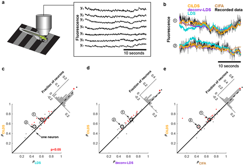
Here we compare the performance of three methods at recovering ground truth latent variables in simulation: one with deconvolution and latent dynamics (CILDS), one with de-convolution but no latent dynamics (CIFA), and one with no deconvolution and no latent dynamics (FA). The simulation parameters are GCaMP6f with 94 neurons and medium noise, as in Fig. 3d. (a) Accuracy of latent variable recovery for CILDS (orange), CIFA (brown), and FA (blue) across a wide range of latent timescales. Note that the R² can be less than zero because these results are cross-validated. The CILDS curve shown here is the same as in Fig. 3d. (b) Mean calcium decay time constant estimated using CILDS (orange) and CIFA (brown) for different simulated latent timescales. FA does not estimate a calcium decay time constant. The dashed black line indicates the ground truth decay time constant. In both panels, coloured error bars indicate standard deviation, and black error bars indicate standard error across n=2000 latent variables (see Methods).

(a) Two-photon calcium imaging using GCaMP6f at 30Hz was performed on three larval zebrafish in a virtual reality environment. Shown are representative fluorescence traces from seven of the imaged neurons. (b) Example recorded fluorescence traces (black) and leave-neuron-out predicted fluorescence using CILDS (orange), deconv-LDS (purple), LDS (cyan), and CIFA (brown). (c-e) Correlation between the recorded fluorescence and the leave-neuron-out predicted fluorescence for CILDS versus each of the other methods. Each point represents one neuron, where the correlation is computed for each trial (27 seconds long), then averaged across all 15 trials. Diagonal histograms show the paired difference in performance between CILDS and one of the other methods, as indicated. The correlation is higher for CILDS than (c) LDS (p = 0.0001, n = 60 neurons, paired two-tailed t-test across the population of neurons, black asterisk indicating statistical significance), (d) deconv-LDS (p = 5.94 × 10⁻⁵, n = 60 neurons), and (e) CIFA (p = 0.046, n = 60 neurons). Note that the histograms are zoomed-in for visual clarity, and therefore the ends of the histograms are not shown. The numbered points (black circles) correspond to the examples shown in panel b. Red points indicate a statistically significant difference per neuron between CILDS and the other method being compared using a paired two-tailed t-test across trials (p < 0.05, see Methods). Note that the threshold used for the t-test means that we might expect 5% of the neurons to appear significant even if the effect is not real.

(a) Two-photon calcium imaging performed on awake mice viewing static gratings with different spatial frequencies and orientations (180 total stimuli) using GCaMP6f at 15.5Hz. Shown are representative fluorescence traces from seven of the imaged neurons. (b) Example segment of recorded fluorescence traces (black) and leave-neuron-out predicted fluorescence traces using CILDS (orange), deconv-LDS (purple), LDS (cyan), and CIFA (brown). (c-e) Correlation between the recorded fluorescence and the leave-neuron-out predicted fluorescence for CILDS versus each of the other methods. Each point represents one neuron, where the correlation is computed for each trial (196.7 seconds long) then averaged across all 15 trials. Diagonal histograms show the paired difference in performance between CILDS and one of the other methods, as indicated. The correlation is higher for CILDS than (c) LDS (p = 5.04 × 10⁻¹⁷, n = 704 neurons, paired two-tailed t-test across the population of neurons, black asterisk indicating statistical significance), (d) deconv-LDS (p = 1.7 × 10⁻²⁷, n = 704 neurons), and (e) CIFA (p = 3.19 × 10⁻⁸¹, n = 704 neurons). Note that the histograms are zoomed-in for visual clarity, and therefore the ends of the histograms are not shown. The numbered points (black circles) correspond to the examples shown in panel b. Red points indicate a statistically significant difference per neuron between CILDS and the other method being compared using a paired two-tailed t-test across trials (p < 0.05, see Methods). Note that the threshold used for the t-test means that we might expect 5% of the neurons to appear significant even if the effect is not real. (f) Flow diagram depicting decoding of visual stimuli using low-dimensional latent variables, which are obtained by applying a dimensionality reduction method to the recorded fluorescence traces. (g) Classification accuracy of the visual stimulus based on latent variables extracted using CILDS (orange), deconv-LDS (purple), and LDS (cyan). Classification was performed using a Gaussian Naive Bayes decoder, where the number of latent variables extracted by each dimensionality reduction method was systematically varied (horizontal axis). There were 180 total gratings (with different orientations and spatial frequencies) shown during the experiment, so the chance classification accuracy is 1/180 (gray dashed). The decoding window was 250 ms, which is the duration of stimulus presentation. Black error bars around the mean indicate 95% confidence intervals (Bernoulli process).